New book on computational biology

Enzyme Kinetics for Systems Biology

by Herbert M Sauro
published at analogmachine.org

------------------------------------------------------------------------

Book summary:

318 pages, 94 illustrations and 75 exercises

This new monograph introduces students to basic reaction kinetics, including enzyme kinetics, cooperativity, allostery and gene regulatory kinetics. The text introduces a number of modern concepts such as generalized rate laws, elasticities and systems biology thermodynamic quantities. The text is suitable for junior undergraduate level in the US and 2nd year undergraduates in the UK. The text can also be used as a reference text for graduates and other researchers. Click here for the Google books preview.

Display Fire!

The simulation tools now display an animated "fire" on top of items after a simulation. The purpose of the fire is to highlight upregulated and downregulated molecules. The size of the fire is proportional to the final output in the simulation.

These fires can be created from Python or Octave scripts using the tc_burn( item, intensity ) command, where intensity is a number in the range (0,1). From C++, a tool can connect to signals in the LabelingTool (in TinkerCellCore library) in order to create these effects.

The fire feature can be completely inactivated from C++ by setting the LabelingTool::ENABLE_FIRE to false.

Events

Events can be inserted using the clock icon in the "Inputs" tab at the top. The events table is stored as part of the "global item", which can be accessed in the command-line using "_". The clock icon can be used to edit the Events. In this screenshot, an event is used with the toggle-switch model to try to switch the toggle-switch from one state to the other (didn't work in this model, because the states are quite robust).

Optimization and Global Sensitivity

TinkerCell now includes optimization functions for fitting time series data and maximizing or minimizing a given formula. The optimization routines are written in Python but use C++ simulators (copasi). The algorithm is Cross Entropy, which can be used to obtain an estimate of the distribution of parameters. PCA can be used to infer global sensitivities.


A user can write any Python function and optimize it using CrossEntropy. Here is template code:

#objective function for CrossEntropy
def MyObjective():
error = 0.0
#do something here, e.g. call tc_getSteadyState or tc_simulateDeterministic
return error

#optimization parameters
minimize = False
maxruns = 100
numPoints = 100
title = "My Optimization Function"

#optimize
result = CrossEntropy.OptimizeParameters(FitFormula_Objective, title, maxruns, numPoints, minimize)
mu = result[0]
sigma = result[1]
paramnames = result[2]
CrossEntropy.DoPCA(mu, sigma, paramnames)

#set the optimized parameters in the model if you want
n = len(mu)
params = tc_createMatrix(n, 1)
for i in range(0,n):
tc_setMatrixValue(params, i, 0, mu[i])
tc_setRowName(params, i, paramnames[i])
tc_setParameters(params,1)

CrossEntropy.DoPCA will generate a summary file such as the one below.

Trying different versions of a model

From Python or Octave, it is relatively simple to try different versions of the same network architecture. For example, the diagram below shows a protein regulating itself. The regulation type is "transcription regulation", i.e. it does not specify whether it is positive or negative regulation. The code below the figure simulates both positive and negative feedback using the tc_substituteModel command.

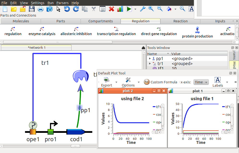
j = tc_find("tr1")

file1 = "/home/deepak/Documents/TinkerCell/Modules/transcription_activation/Equilibrium_Model.tic"

file2 = "/home/deepak/Documents/TinkerCell/Modules/transcription_repression/Equilibrium_Model.tic"

tc_multiplot(2,1)

tc_substituteModel(j, file1)

m1 = tc_simulateDeterministic(0,100,100)

tc_plot(m1, "using file 1")

tc_substituteModel(j, file2)

m2 = tc_simulateDeterministic(0,100,100)

tc_plot(m2, "using file 2")

It is also possible to practically remove a component from the model by substituting "empty" for the model, e.g. tc_substituteModel(j, "empty")

Converting models to English

The semantics used in TinkerCell allows conversion of a model into plain English. The Export menu has this feature. Below is an example:

Model:

English export:

transcription factor (repressor) LacI represses repressor binding site (target) lac_op

transcription factor (repressor) TetR represses repressor binding site (target) tet_op

coding (template) gfp_gene produces reporter (product) GFP

molecule (inhibitor) IPTG inhibits transcription factor (target) LacI

molecule (inhibitor) aTc inhibits transcription factor (target) TetR

coding (repressor) gene represses repressor binding site (target) op3

Automatically iterating through models

The same "diagram" can be modeled in different ways. So, what is the consequence of the type of model we pick? The new python plugin called tryAllModules.py plots the simulation of all the combinations of submodels and then clusters the results, showing a picture of how the system can behave depending the modeling methods used.



The key functions used by the python code are:

tc_listOfPossibleModels
tc_substituteModel
tc_holdPlot
tc_clusterPlots

Important note: The load model function in TinkerCell caches each model that is loaded. The caching checks if the file has changed. In file has not changed, the re-loading of the same model is very fast, since it does not need to parse the file itself. This results in an order or magnitude speed up when doing tc_substituteModel repeatedly.

Sample Python Code for Creating a Little Network

cds4 = tc_insert("cds4","Coding")
p3 = tc_insert("p3","Inducible Promoter")
cds3 = tc_insert("cds3","Coding")
t3 = tc_insert("t3","Terminator")
p2 = tc_insert("p2","Inducible Promoter")
cds2 = tc_insert("cds2","Coding")
t2 = tc_insert("t2","Terminator")

listOfParts = [cds4, p3, cds3, t3, p2, cds2, t2]
tcArray = toTC(listOfParts) #convert Python data structure to

tc_alignParts(tcArray)

#production of P4
P4 = tc_insert("P4", "Transcription Factor")
x = tc_getX(cds4)
y = tc_getY(cds4)
tc_setPos(P4, x, y - 200)

listToConnect = [cds4, P4]
tcArray = toTC(listToConnect)
R1 = tc_insertConnection(tcArray, "R1", "Protein Production")

#P4 regulates p3

listToConnect = [P4, p3]
tcArray = toTC(listToConnect)
R2 = tc_insertConnection(tcArray, "R2", "Transcription Activation")

#production of P3
P3 = tc_insert("P3", "Transcription Factor")
x = tc_getX(cds3)
y = tc_getY(cds3)
tc_setPos(P3, x, y - 200)

listToConnect = [cds3, P3]
tcArray = toTC(listToConnect)
R3 = tc_insertConnection(tcArray, "R3", "Protein Production")

#P3 regulates p2

listToConnect = [P3, p2]
tcArray = toTC(listToConnect)
R4 = tc_insertConnection(tcArray, "R4", "Transcription Activation")

#production of GFP
GFP = tc_insert("GFP", "Reporter")
x = tc_getX(cds2)
y = tc_getY(cds2)
tc_setPos(GFP, x, y - 200)

listToConnect = [cds2, GFP]
tcArray = toTC(listToConnect)
R5 = tc_insertConnection(tcArray, "R5", "Protein Production")

Testing different modeling methods easily

The following Python code was tested on the ComK_ComS example file. It generates all possible modeling methods for connections ta1 and pp2, which are transcription regulation and protein production connections.

ta1 = tc_find("ta1")

pp2 = tc_find("pp2")

models1 = tc_listOfPossibleModels(ta1)

models2 = tc_listOfPossibleModels(pp2)

tc_multiplot(models2.length, models1.length)

for i in range(0,models1.length):

tc_substituteModel(ta1, tc_getString(models1,i))

for j in range(0,models2.length):

tc_substituteModel(pp2, tc_getString(models2,j))

m = tc_simulateDeterministic(0,100,100)

tc_plot(m, "sys" + str(i*j+1))

There are two different ways to model transcription regulation in the current TinkerCell repository. There are three different ways to model protein production in the current repository. So, there are 6 possible combinations. The following graphs were the output of the python code.

Operator sites

"Operator" has been added as a new part type. It has sub-families called "Activator Binding Site" and "Repressor Binding Site". An Inducible Promoter is defined as a combination of an Activator Binding Site and a Promoter part. A Repressible Promoter is defined as a combination of Repressor Binding Site and Promoter. Only one transcription factor is allowed to bind to a single operator site -- this makes modeling much more convenient, but it also makes sense physically.